Long time, no see: Virtual Lunch Roulette
Abstract:
When distributing individuals into groups every week for a virtual social mixer, e.g. using Zoom breakout rooms, it’s boring to end up in a group with someone, who you already met last week. We compute the probility for this to happen and state a simple rejection sampling proposal for how to increase social diversity in such groupings.

 This work is licensed under a Creative Commons
Attribution-ShareAlike 4.0 International License. The R-markdown
source code of this blog is available under a GNU General Public
License (GPL v3) license from GitHub.
Introduction
As a pandemic replacement for the cross-division-chance-encounter in the coffee kitchen, it has become common to use a virtual social mixer format, where the \(n\) participants are randomly divided into groups of at least \(m\) people, e.g., for a video meeting or Zoom breakout rooms. Software exists to institutionalize such Random Lunches for, e.g., Slack. In this post we shall be interested in the properties of such group assignment algorithms.
A practical experience is that all too often, the algorithm assigns me to a group where at least one of the participants was already in my group the last time. Before accusing the programmers of writing a poor grouping algorithm: can we determine mathematically what the probability for such a “reunion” is? How can we modify the algorithm to avoid this?
Survey of the field
Arranging a fixed set of \(n=k\times m\) individuals into \(k\) groups of size \(m\) in subsequent rounds ensuring that no overlap occurs between the groups for as many rounds as possible is also known as the social golfer problem or round robin scheduling in combinatorics - and can be solved using constraint programming. Compared to the social golfer problem, we have the additional challenge that the group of people between rounds may be subject to change. Furthermore, \(m\) might not be a divisor of \(n\). Hence, somewhat closer to our problem is the so called maximally diverse grouping problem, where the grouping is to be done such that the requirements on group size are met and a diversity score over the elements in each group is maximized. For our setup, the score could, e.g., be time since the last meet between individuals. Integer programming can be used to solve the NP-complete problem.
However, in our application we will either ignore the diversity score altogether (i.e. set it to 1 always) or use a 0/1 diversity score (met last time or not). Furthermore, we are interested in random assignment algorithms selecting uniformly among the valid configurations. As a consequence, we choose a more probabilistic approach and instead use a custom group assignment algorithm as described in the next section.
The Grouping
We want to split the \(n\)
individuals into groups of preferably \(m\) members. However, if \(m\) is not a divisor of \(n\) then after making \(\lfloor n/m \rfloor\) groups of \(m\) members we would have \(l = n - \lfloor n/m \rfloor\) individuals
left. Instead of assigning these to a single leftover group, which would
be of size less than \(m\)
(particularly critical is size 1), we assign the remaining individuals
to the \(l\) groups in round robin
fashion. This ensures that each group has size at least \(m\). Note: Depending on \(n\) and \(m\) the resulting sizes might be larger
\(m+1\), but the difference in the
resulting group size will never be larger than 11.
Let people be a tibble with a column id
denoting a primary identifier key - this could, e.g., be the people’s
email address. An R function to perform a random assignment of the \(n\)=nrow(people) individuals
into groups of at least \(m\) could
look like:
#' Sample people into groups (original algorithm)
#'
#' @param people tibble containing name and email of available ppl
#' @param m requested group size. If m not a divisor of nrow(people) then put leftovers in existing groups
#'
#' @return A list of vectors where each vector containing the ids (row number in ppl) of those belonging to the same group
#'
sample_groups <- function(people, m) {
  # Number of groups needed
  n_g <- nrow(people) %/% m
  # Group membership indicator
  g <- rep(seq_len(n_g), length.out=nrow(people))
  # Permutation order
  perm <- sample(seq_len(nrow(people)))

  # Make a list of ids in each group
  groups <- map(seq_len(n_g), function(i) {
    idx <- perm[which(g == i)]
    people %>% slice(idx) %>% pull(id)
  })

  return(groups)
}
Example: Let people denote the population of 47
individuals to be assigned into groups of at least \(m=4\) according to the above
description.
n <- 47
people <- tibble(id = str_c("id", sprintf("%0.2d",seq_len(n))))
m <- 4
groups <- sample_groups(people, m=m)
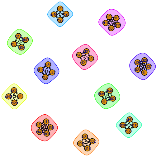
This leads to 11 groups with between 4 and 5 members. We can visualize the group allocation as a graph, where each group will correspond to a fully connected sub-graph, but with no connections between the sub-graphs.

Mathematical Formulation
The mathematical question is now: Given you were in the group with \(l\) other persons the last time, what is the probability that after assigning \(n\) individuals into groups of preferred size \(m\geq 2\), that you will be in the same group with at least one of them again this time2. Let \(m \leq k\) be the size of your group in the current assignment. Combinatorical considerations tell us the probability to meet at least one of the \(l\) persons again is:
\[ p(k, l, n) = 1 - \frac{1\cdot\prod_{i=2}^{k} (n-(l+i-1))}{1\cdot\prod_{i=2}^{k} (n-i+1)}. \] In order to determine the overall probability for a reunion after assignment, we need to determine the PMF \(f_{n,m}\) of the group size, i.e. what is the probability that the algorithm dividing \(n\) individuals into groups of size at least \(m\) will assign me to a group of size \(k, k\geq m\). The probability of interest is then: \[ p(n,m,l) = \sum_{k=1}^\infty p(k,l,n) f_{n,m}(k) \] Note: Even though we write the summation to be from 1 to \(\infty\), the PMF will only have support on at most two integers.
The calculations in R and verified by 1000 Monte Carlo simulations:
# Group membership indicator for the n individuals
g <- rep(seq_len(n %/% m), length.out=n)

# Which previous group sizes to consider. Note:
# can be way beyond m, even if m was selected
p_groupsize <- prop.table(table(table(g)))

p_kln <- sapply(as.numeric(names(p_groupsize)), prob_reunion, l=l, n=n)
c(p_analytical = sum(p_kln * p_groupsize), p_mc = p_reunion_mc)
## p_analytical p_mc
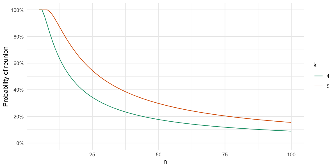
## 0.2024913 0.2010000We can illustrate this reunion probability as a function of \(k\) and \(n\).

As a next step we need to marginalise out the previous group size \(l+1\). For simplicity, we will assume that exactly the same participants participate in each round. Hence, we can use the same group size PMF as before when summing out \(l\): \[ p(n,m) = \sum_{l=1}^\infty \sum_{k=1}^\infty p(k,l,n) f_{n,m}(k) f_{n,m}(l+1) \]
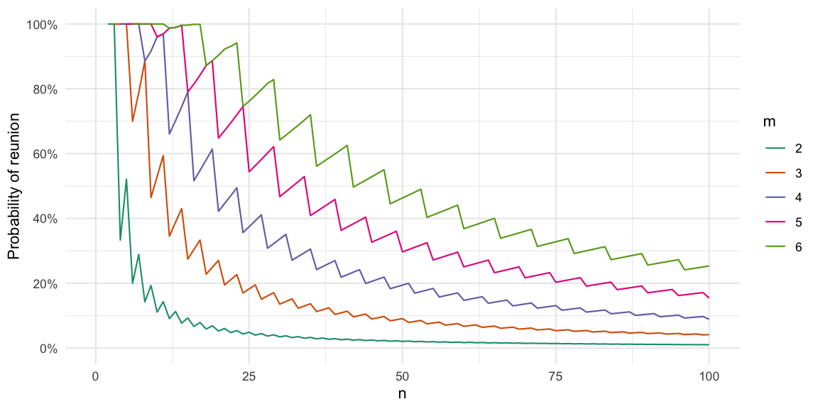
The result thus denotes the probability that you in two consecutive assigments of \(n\) individuals into groups of at least \(m\) individuals will be in the same group with someone twice. We will denote this the reunion probability. The graph below shows this probability as a function of \(n\) and \(m\) and is also available in a log-x axis version.

Why are the curves not decreasing monotonically?3 This is due to the minimum size \(m\) restriction on the group size. If \(m=6\) and you have \(n=12\) people then there are two groups. But if \(n=17\) while \(m\) is still 6, then we will still only have two groups as one would need 18 people for 3 groups. However, there are now 8 and 9 people in the two groups instead of 6 and 6 so the probability of reunion increases. Altogether, the probability increases from 12 and 17 until it decreases again at \(n=18\). Consequently, for \(m=2\) the peaks would be at the even \(n\) and the troughs would be the odd \(n\).
Given our \(n=47\) and \(m=4\) we also note the high probability of 22% for a reunion, which confirms our empirical experience. Thus there seems to be a need to impose some additional constraints on the grouping in order to optimize social diversity. For a translation of \(m\) into the number of breakout rooms used in Zoom, see Appendix A.
Grouping with avoidance
Let pairs be a tibble with columns id1 and
id2 denoting all pairs of individuals who were placed in
the same group the last time. We now want to enhance our group
allocation algorithm to only assign people into groups, if they were not
in the same group the last time. We do this by a simple rejection
sampling algorithm, where we draw a configuration with
sample_groups, check if it has overlaps with the last
allocation, and if so, draw again. This method is not very efficient and
might take a while. Even worse: it might not finish at all, if no
configuration satisfying the constraint exist. An example is, if 9
individuals are to be divided into groups of at least 4 two times
without any reunions. The corresponding code of such a
sample_groups_avoid function is available in the R
code from GitHub. This can then be used to generate the desired
grouping without reunions:
# Sampling in round1 and round2
groups_r1 <- sample_groups(people, m=m)
groups_r2 <- sample_groups_avoid(people, m=m, avoid_pairs = make_pairs(groups_r1))

# Check if there are any re-unions. Note: There should be none.
inner_join( make_pairs(groups_r1) %>% select(hash), make_pairs(groups_r2) %>% select(hash), by="hash")
## # A tibble: 0 x 1
## # … with 1 variable: hash <chr>In other words: No reunions, just as we wanted.
Discussion
We considered random groupings used, e.g., in lunch roulette or when distributing students into breakout rooms. Depending on the number of people to group and the anticipated group size the probability for a reunion with somebody from last weeks grouping is surprisingly high. Hence, we use rejection sampling to propose a configuration, where no reunion occurs. The resulting grouping can easily be exported to a CSV file for import when making pre-assigned Zoom breakout rooms (example in the R code on GitHub). Even better allocations might be possible as part of solving the maximally diverse grouping problem. For further combinatorics posts, see also my work on the birthday problem with unequal probabilities.
Acknowledgments
Thanks to Dirk, Titus and Filip for the challenge.
Appendix A
Since the Zoom grouping does not work by specifying the number of
individuals in each group, but instead the number of groups, we show an
equivalent representation of the reunion probability graph as a function
of the number of groups, i.e. \(\lfloor
n/m\rfloor\). Since we did the math in \(m\), not every breakout room size is found.
This also means that the shown graph is only an approximation, because
the Zoom allocation algorithm is likely to work slightly different to
our proposed sample_groups algorithm.

Appendix B
As a consequence from the calculation and functions from this post we can now answer the following question from our SU Mathematical Statistics Zoom Christmas Party announcement:
Through simulations (details in the code)
built on top of the sample_groups function we determine
that the requested probability when \(n=30\) participate in the X-mas party is
7.6%.
Literature
As an example consider the case \(n=7\) and \(m=4\), where we according to our specification would form 1 group with 7 members.↩︎
We will assume that the \(l\) individuals you met last week all participate again this week.↩︎
Thanks to u/antichain for the question and to u/assiraN for the nice answer with examples, which I’ve integrated into the post.↩︎