Speedmining the Cubing Community with dbplyr
Abstract:
We use the RMariaDB and dbplyr packages to
analyze the results database of the World Cubing Association. In
particular we are interested in finding unofficial world records of
fastest 3x3x3 solves, countries with large proportion of female cubers
as well as acceptable solving times before entering a WCA
competition.
 This work is licensed under a Creative Commons
Attribution-ShareAlike 4.0 International License. The
markdown+Rknitr source code of this blog is available under a GNU General Public
License (GPL v3) license from github.
This work is licensed under a Creative Commons
Attribution-ShareAlike 4.0 International License. The
markdown+Rknitr source code of this blog is available under a GNU General Public
License (GPL v3) license from github.
Motivation
An item on my bucket list of irrelevant-things-to-excel-in-during-parental-leave™ is to solve the Rubik’s cube again. In 2013 I learned the beginner’s method for solving the cube by reading Dan Harris’ Speedsolving the Cube book. However, any attempts to improve times by learning CFOP failed miserably in 2013 due to lack of time. So in this 2019 attempt I just try to revoke my beginner’s method and improve it slightly by 4LL. Nevertheless, my solves fluctuate at 120-180s. This has made me worry about the shame-factor of pulling through the next item on the bucket list: competing in a World Cubing Association (WCA) 3x3x3 competition. The motivating question of this post is therefore: how large a skill outlier would one be at such a competition with, say, an 180s average?
Mining the World Cubing Association Database
Luckily, the WCA provides the results of all cubers and competitions
in a downloadable
SQL database (400 MB mySQL/MariaDB SQL text file). The downloadable
version of 19 Apr 2019 contains tables with information on all 124,997
players, 6,014 competitions as well as the 2,130,374 results obtained by
players in competitions starting with the Rubik’s Cube World
Championship in 1982. Not big data, but big enough
and structured in a way that justifies using a SQL database backend for
the analysis instead of just a flat data.frame in R.
With a little bit of effort, one installs a MariaDB together with the MariaDB
Connector/C and imports the WCA data into the database.
Subsequently, the RMariaDB (Müller et al. 2018) and DBI
(R Special Interest Group on
Databases (R-SIG-DB), Wickham, and Müller 2018) R packages allow
one to connect directly to the DB. Furthermore, the dbplyr
(Wickham and Ruiz
2019) package allows one to write dplyr code, which
is then translated into and evaluated as SQL queries behind the
scenes.
We connect to the database as follows:
library(DBI)
library(RMariaDB)
con <- DBI::dbConnect(RMariaDB::MariaDB(), group="my-db")
where, as suggested in the RMariaDB
package documentation, my-db is a custom group defined
in the option file ~/my.cnf containing the user, password,
protocol type and the database to use (wca). This is
preferred instead of calling dbConnect with options such as
socket, user, password and
dbname.
To import the data one can either open a mysql shell and
type SQL commands or send the SQL query from R to the database:
SOURCE WCA_export.sql;After such an import we can view the contents of the database:
dbListTables(con)## [1] "eligible_country_iso2s_for_championship" "Formats" "Countries"
## [4] "RoundTypes" "Rounds" "Competitions"
## [7] "Continents" "Persons" "championships"
## [10] "Events" "Scrambles" "RanksAverage"
## [13] "Results" "RanksSingle"Of particular interest is the Results table, where each
row contains the results of a player (personId) in a round
of a WCA competition of events such as the 2x2x2, 3x3x3, 4x4x4, etc. For
the 3x3x3
event each round consist of five solves solves
(values1-values5) of which the best is
reported in the column best and the trimmed mean (removing
the best and worst solve and computing the mean of the three other
solves) is reported in the column average.
##  [1] "competitionId"         "eventId"               "roundTypeId"           "pos"                   "best"                  "average"
##  [7] "personName"            "personId"              "personCountryId"       "formatId"              "value1"                "value2"
## [13] "value3"                "value4"                "value5"                "regionalSingleRecord"  "regionalAverageRecord"
Furthermore, the table Personscontains additional basic
information about each player:
## [1] "id" "subid" "name" "countryId" "gender"Note: At WCA competitions there is no separate ranking according to gender.
After getting initially acquainted with the database, we do two small
SQL-side modifications. The first modification is to create an index for
the tables, which will help to substantially reduce the join times later
on. The second is to merge the separate year, month, day columns of the
event day in the Competitions table into a single ISO 8601
date. See the github
code for details.
As the next step we create tables to use with dbplyr.
These will then just dispatch to the database tables. For now, we work
only with the results of the 3x3x3 cubes, but will join the Results,
Persons and Competitions table in order to get relevant information
about gender of the person as well as date of the solve together with
the time of each solve.
suppressPackageStartupMessages(library(dbplyr))
suppressPackageStartupMessages(library(dplyr))

results <- tbl(con, "Results") %>% filter(eventId == "333")
persons <- tbl(con, "Persons")
competitions <- tbl(con, "Competitions2")

##JOIN the three tables together
allResults <- results %>% inner_join(persons, by=c("personId"="id")) %>%
  inner_join(competitions, by=c("competitionId"="id"))
Note that dbplyr uses lazy evaluation, i.e. calls are
not executed before needed. However, one can with
show_query check the SQL call, which is used in case of
evaluation. In this example the SQL query to get the results of female
cubers, i.e.:
fwr_single <- allResults %>% filter(gender == "f", best>0)in SQL looks like
fwr_single %>% show_query()## <SQL>
## SELECT *
## FROM (SELECT `LHS`.`competitionId` AS `competitionId`, `LHS`.`eventId` AS `eventId`, `LHS`.`roundTypeId` AS `roundTypeId`, `LHS`.`pos` AS `pos`, `LHS`.`best` AS `best`, `LHS`.`average` AS `average`, `LHS`.`personName` AS `personName`, `LHS`.`personId` AS `personId`, `LHS`.`personCountryId` AS `personCountryId`, `LHS`.`formatId` AS `formatId`, `LHS`.`value1` AS `value1`, `LHS`.`value2` AS `value2`, `LHS`.`value3` AS `value3`, `LHS`.`value4` AS `value4`, `LHS`.`value5` AS `value5`, `LHS`.`regionalSingleRecord` AS `regionalSingleRecord`, `LHS`.`regionalAverageRecord` AS `regionalAverageRecord`, `LHS`.`subid` AS `subid`, `LHS`.`name` AS `name.x`, `LHS`.`countryId` AS `countryId.x`, `LHS`.`gender` AS `gender`, `RHS`.`name` AS `name.y`, `RHS`.`cityName` AS `cityName`, `RHS`.`countryId` AS `countryId.y`, `RHS`.`information` AS `information`, `RHS`.`year` AS `year`, `RHS`.`month` AS `month`, `RHS`.`day` AS `day`, `RHS`.`endMonth` AS `endMonth`, `RHS`.`endDay` AS `endDay`, `RHS`.`eventSpecs` AS `eventSpecs`, `RHS`.`wcaDelegate` AS `wcaDelegate`, `RHS`.`organiser` AS `organiser`, `RHS`.`venue` AS `venue`, `RHS`.`venueAddress` AS `venueAddress`, `RHS`.`venueDetails` AS `venueDetails`, `RHS`.`external_website` AS `external_website`, `RHS`.`cellName` AS `cellName`, `RHS`.`latitude` AS `latitude`, `RHS`.`longitude` AS `longitude`, `RHS`.`date` AS `date`
## FROM (SELECT `LHS`.`competitionId` AS `competitionId`, `LHS`.`eventId` AS `eventId`, `LHS`.`roundTypeId` AS `roundTypeId`, `LHS`.`pos` AS `pos`, `LHS`.`best` AS `best`, `LHS`.`average` AS `average`, `LHS`.`personName` AS `personName`, `LHS`.`personId` AS `personId`, `LHS`.`personCountryId` AS `personCountryId`, `LHS`.`formatId` AS `formatId`, `LHS`.`value1` AS `value1`, `LHS`.`value2` AS `value2`, `LHS`.`value3` AS `value3`, `LHS`.`value4` AS `value4`, `LHS`.`value5` AS `value5`, `LHS`.`regionalSingleRecord` AS `regionalSingleRecord`, `LHS`.`regionalAverageRecord` AS `regionalAverageRecord`, `RHS`.`subid` AS `subid`, `RHS`.`name` AS `name`, `RHS`.`countryId` AS `countryId`, `RHS`.`gender` AS `gender`
## FROM (SELECT *
## FROM `Results`
## WHERE (`eventId` = '333')) `LHS`
## INNER JOIN `Persons` AS `RHS`
## ON (`LHS`.`personId` = `RHS`.`id`)
## ) `LHS`
## INNER JOIN `Competitions2` AS `RHS`
## ON (`LHS`.`competitionId` = `RHS`.`id`)
## ) `dbplyr_001`
## WHERE ((`gender` = 'f') AND (`best` > 0.0))Analysing the data
We are now all ready to perform some descriptive analyses of the data. The top-5 females according to their time for 3x3x3 single solve is obtained by:
fwr_single %>%
  group_by(personId) %>% top_n(-1, best) %>% ungroup %>%
  arrange(best) %>%
  select(competitionId, personName, personCountryId, best, date) %>%
  top_n(-5, best)
## # Source: lazy query [?? x 5]
## # Database: mysql 10.3.14-MariaDB-log [hoehle@localhost:/wca]
## # Ordered by: best
## competitionId personName personCountryId best date
## <chr> <chr> <chr> <int> <date>
## 1 SlowNSteadySummer2017 Dana Yi USA 537 2017-07-01
## 2 BarbyCubeOpen2018 Juliette Sébastien France 581 2018-11-03
## 3 FruitSalad2018 Katie Hull USA 606 2018-03-03
## 4 CubeduKorea2018 Yu Da-Hyun (유다현) Korea 629 2018-01-26
## 5 NewYorkCitySpring2018 Kymberlyn Calderon USA 641 2018-04-21Note that the solve times are given in centiseconds (i.e. 1/100’th of a second). The above result can be compare with the corresponding information at https://wcadb.net.
As professional data scientist one knows how important it is to understand the data generating process and to know your data. So this is how the 5.37s solve by Dana Yi in 2017 looks like:
The evolution of the 3x3x3 single solve WR
So at this point we force an execution of the allResults
query and cache the result as an object in R. This feels slightly
disappointing, because the hope was to leave the data in the database
management system (DBMS) as long as possible, but it felt like the most
efficient way to compute sequential ranks - however, it might have been
possible to perform the sequential rank directly using SQL statements,
although I did not succeed to find the correct approach within the
available time 1.
Instead, the results are sorted according to their date in R and
subsequently each result is checked to see if it’s sequential rank is 1,
i.e. whether the time is lower than all previous results. For this
purpose a fast Rcpp function sequential_is_rank1 function
is provided, which computes the sequential rank of a vector of values
(see github
code for details). Note: If we had not pulled the data into R at
this point, such a computation within R would not have been
possible.
The evolution of the world record for males and females over time is then easily plotted. Note: As mentioned WCA doesn’t officially distinguish between male and female results.
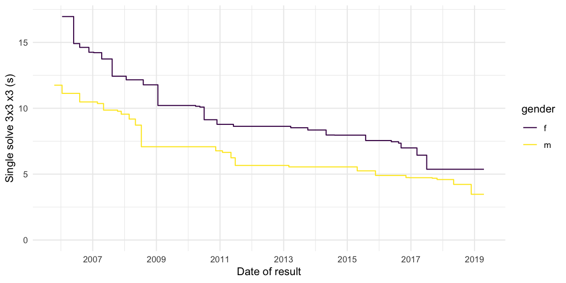 Is such a plot useful? Not really IMHO, but I had seen a similar plot at
the WCA
webpage, so it’s nice to be able to create it in R.
Is such a plot useful? Not really IMHO, but I had seen a similar plot at
the WCA
webpage, so it’s nice to be able to create it in R.
Countries with highest proportion of female cubers
Since the overall fraction of female cubers is around 10%, we
determine the top-5 countries (with at least 50 cubers), having the
highest proportion of female cubers in the Persons
database:
| countryId | n_total | n_male | n_female | frac_female (in %) |
|---|---|---|---|---|
| Algeria | 157 | 103 | 54 | 34.4 |
| Mongolia | 373 | 278 | 95 | 25.5 |
| Morocco | 67 | 53 | 14 | 20.9 |
| Pakistan | 54 | 42 | 12 | 22.2 |
| Tunisia | 211 | 171 | 40 | 19.0 |
I find this list quite surprising and also encouraging!
Skill level before entering a WCA competition
Getting back to the motivating question of this post, we derive for each result how experienced the cuber was at the time of obtaining the result. We shall measure experience terms of years since the cuber’s first WCA competition. Special interest will then be in results of cubers in their very first WCA competition - see the github code for details.
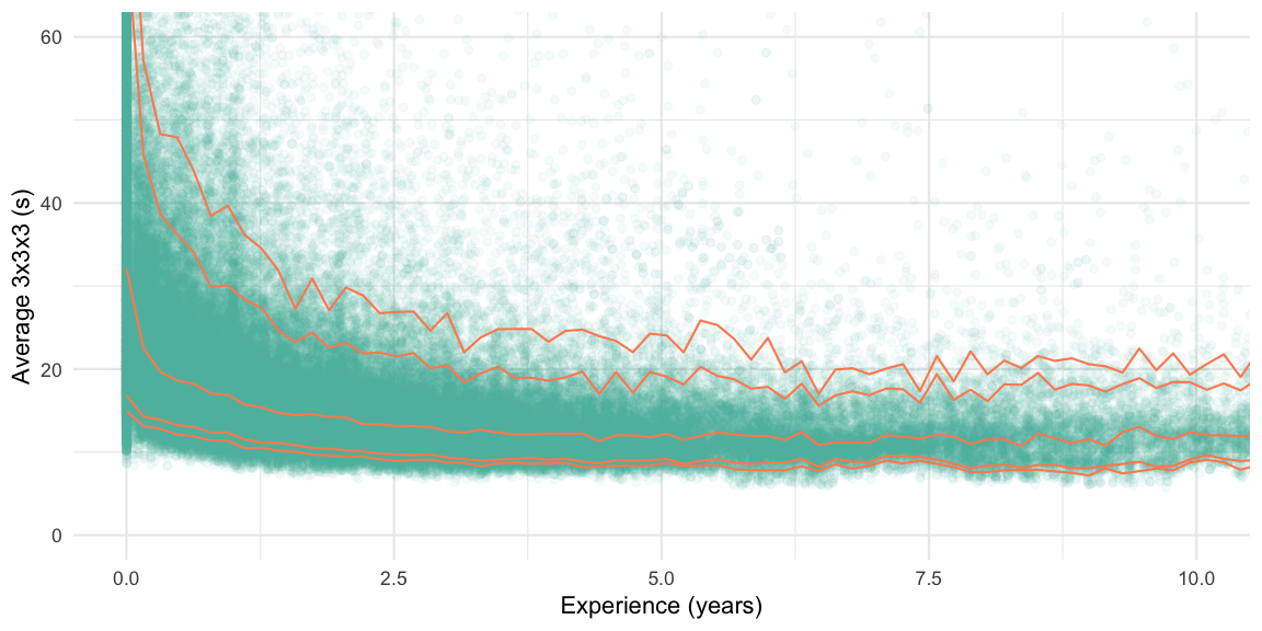
We then use this information to create a scatter plot with result
average (in seconds) and corresponding experience of the cuber (in
years). For better visualization we plot the marginal 5%, 10%, 50%, 90%,
95% quantiles as smooth function of experience - this is done with with
ggplot2’s geom_quantile function together with
the argument method="rqss", which then uses the
rqss function of the quantreg package (Koenker 2018) to compute
smooth quantile curves:
We notice that the quantile curves stay more or less parallel, which is
indicative of a stable variance and skewness of the results over the
range of experiences. Focusing only on the round-1 results of those
participating for the first time in the period from 2018-04-19 to
2019-04-19 we see that the quantiles for the average is (in seconds)
are:
##    5%   10%   50%   90%   95%   99% 99.9%
##    16    19    36    77    93   136   208
This shows that with a 180s average one is located at the 99.7% quantile of all cubers entering a WCA competition. In other words: if the comfort zone is defined as being within the 95% envelope, then a ~90s average is needed before entering a WCA competition.
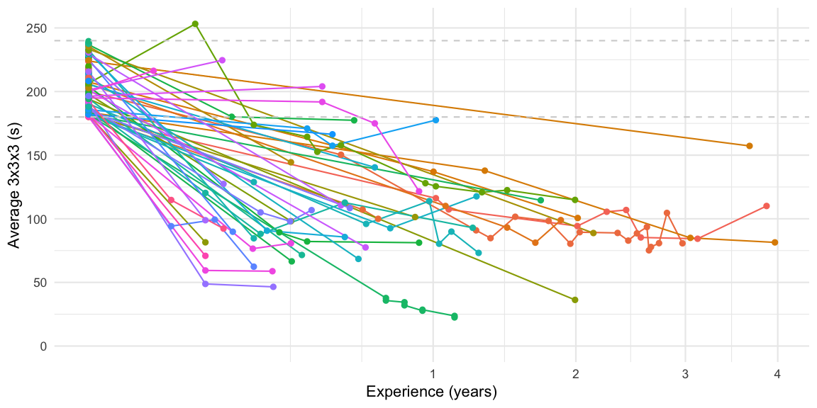
To further investigate, how cubers of that skill level evolve in time, we study the solving skills of cubers entering their first WCA competition with a solve time between 180s and 240s. In order to reduce the potential effect of secular trends due to, e.g., better cubes, we consider the skill evolution of the cohort of first time cubers from 2015 and onwards.
The cohort inclusion criterion provide a total of 168 first time competitors in this skill bracket. Only 28.0% of these cubers decide to participate in further WCA competitions! The further development of the averages of these cubers is best shown in a trajectory plot. Note that the end of the lines does not necessarily mean that they stopped cubing, instead it could be due to right truncation, because only competitions until 2019-04-19 are available.
 Instead of the trajectories we can also overlay an expectation smoother
on top of the data to see how the expected average progresses with time
in the cohort. Note, that this portrays the marginal expectation and
thus is only based on cubers, who are still cubing at that time. No
adjustment for any, potentially informative, drop-out is made.
Instead of the trajectories we can also overlay an expectation smoother
on top of the data to see how the expected average progresses with time
in the cohort. Note, that this portrays the marginal expectation and
thus is only based on cubers, who are still cubing at that time. No
adjustment for any, potentially informative, drop-out is made.
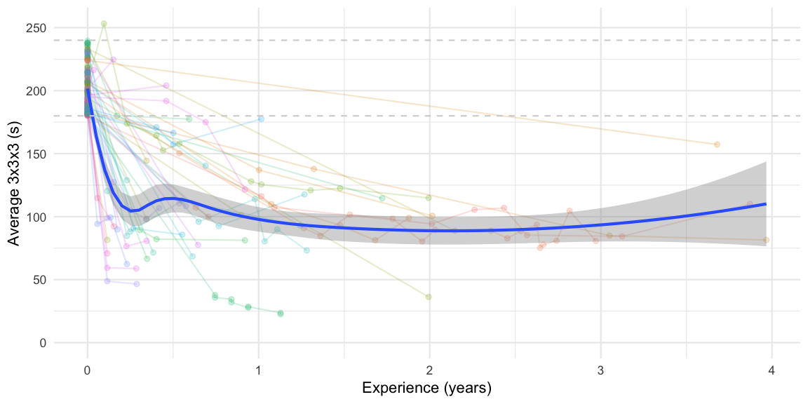
From the figure we notice a rapid improvement the first 6 months after entering the first WCA competition. Hereafter results only improve slowly.
Discussion
Through analysis of the WCA results database it became clear that
participating in a 3x3x3 event with a 180s average is uncool
2 does not take you to winners’
rostrum 3. The data also show that cubers
entering the world of WCA competitions with such an average are likely
to never participate in another WCA event. In case they do, their times
drop to 90-120s averages within 6 months after which they are stuck - it
is very unlikely that they will crack the 20s barrier. To conclude: In
my situation it seems wise to practice more, before going to the first
WCA competition. 😃
From a data science perspective this post provided insights on using
dbplyr as a tidyverse frontend for SQL queries. Being an
SQL novice, I learned that generating indexes is a must, if you
do not want to wait forever for your INNER JOINs. Furthermore,
I ran into some trouble with mutates and filters with the package,
because the produced SQL code provide empty results. It remains unclear
to me if this was due to differences in SQL DBMSs (e.g. MariaDB being
differnet from PostGres), my lack of SQL knowledge or if it’s a
shortcoming of the dbplyr package. My conclusion is that
performing the data wrangling within the DBMS was overkill for the
medium sized wca data. For larger or more structured datasets such an
approach can, however, be fruitful, because a DBMS’s main purpose is to
provide efficient solutions for working with your data. Furthermore, I
like the idea of having a familiar dplyr frontend and just auto-generate
an efficient backend code (here: SQL) to do the actual wrangling. This
also provides an opportunity to get an outside-R-implementation, which
can be an important aspect in quality
assurance of statistical analyses.
Acknowledgments
The terms of use of the WCA database requests any use of it to be equipped with the following text:
This information is based on competition results owned and maintained by the World Cube Association, published at https://worldcubeassociation.org/results as of April 19, 2019.
Besides this formal note, I thank the WCA Results Team for providing the WCA data for download in this comprehensive form!
Literature
If you know how to do this efficiently in SQL, let me know!↩︎
- A reddit user correctly pointed out that just because your
results are at the low end does not necessarily imply that it is
uncool to participate in a WCA competition:
Card
This is very true and I’ve updated the post accordingly. However, if you like me already are an age outlier while your kid is too young to act as your alibi companion, I miss the courage to also be a total skill outlier… But that’s my problem and just motivates me to train more (if time permits) before signing up. 😏↩︎
From readings on speedsolving.com I now learned that there exist (partial) 40+ rankings, which can help to assess the skill level in that age bracket in more detail. My interest was in the skill level of the overall cubing population though.↩︎