The Olympic Medal Table Visualized Gapminder Style
Abstract
Following Hans Rosling’s Gapminder animation style we visualize the total number of medals a country wins during each olympic summer games in relation to the country’s gross domestic product (GDP) per capita. We illustrate how R’s data wrangling capabilities provide a useful toolbox to make such an analysis happen.
 This work is licensed under a Creative Commons
Attribution-ShareAlike 4.0 International License. The
markdown+Rknitr source code of this blog is available under a GNU General Public
License (GPL v3) license from github.
This work is licensed under a Creative Commons
Attribution-ShareAlike 4.0 International License. The
markdown+Rknitr source code of this blog is available under a GNU General Public
License (GPL v3) license from github.
Introduction
Long Swedish winter nights are best spent watching Hans Rosling’s
inspiring TED
talks. Such visualizations help the statistician make points about
temporal trends in a x-axis to y-axis relationship, which otherwise
might drown in modelling details. Recently, I stumbled over a blog post on
how to use the gganimate R
package to animate the Gapminder data available from the
gapminder package. In order to perform a similar
Rosling style animation consider the following: Today, the
Olympic Summer Games in Rio de Janeiro end. As usual this spawns a
debate, whether the nation’s participation has been successful. For this
purpose the olympic medal
table is often taken as basis for comparisons, e.g., to mock your neighbouring
countries. Recent analyses and visualization have been interested in
how to correct these tables for, e.g., population size or, more
interesting, analyse the influence of GDP. For example:
- Google provides alternative Olympics medal tables
- Time Magazine discusses whether it is fair to rank countries by medals achieved alone
The aim of the present blog note is to visualize how countries perform in the medal table in relation to their GDP per capita. From a technical viewpoint we experiment with using R to scrape the olympic medal tables from Wikipedia and animate the results Gapminder style. Disclaimer: We only show the potential of such an analysis and, hence, worry less about the scientific validity of the analysis.
Data
We use the data of Gapminder in order to obtain country specific population and GDP per capita data for each of the years in the period of 1960-2016. The olympic medal tables are ‘harvested’ from Wikipedia.
Olympic medal tables
Olympic medal tables were extracted using the rvest
package from the corresponding Wikipedia pages by using
table-extracting-code described in the post by Cory
Nissen. The Wikipedia tables contain the current state of the medal
table and hence take changes in the medal distribution, e.g. deprivation
due to doping, into account. For details on such a table, see for
example the medal
table of the 2012 summer games in London. In order to stay focused
we hide the scraping functionality in the function
scrape_medaltab - see the code on GitHub for more
details.
#Years which had olympic games
olympic_years <- seq(1960, 2016, by=4)

# Extract olympic medal table from all olympic years since 1960
medals <- bind_rows(lapply(olympic_years, scrape_medaltab))

# Show result
DT::datatable(medals)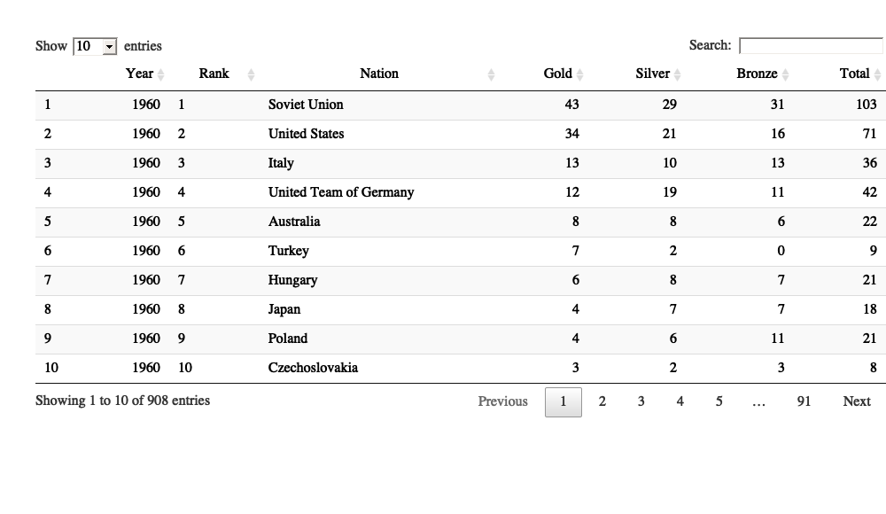
Gapminder data
We obtain GDP per capita and population data from Gapminder. Unfortunately,
these need to be fetched and merged manually. A more convenient way
would have been to take these directly from the package gapminder,
but newer GDP data
are now available. Again, we hide the details of the data wrangling
activities and refer to GitHub code.
For convenience, we also extract the corresponding continent each
country belongs to. This can be done conveniently by comparing with the
gapminder dataset (see code for details).
Joining the two data sources
In principle, all that is left to do is to join the two data sources using the country name of the gapminder dataset and the nation names of the olympic medal tables. However, a challenge of the present country based analysis is how to incorporate the many political changes which happened during the analysis period. As an example, East Germany participated as independent national olympic committee during 1968-1988, but the gapminder data only contain GDP data for Germany as a total. We therefore aggregate the results of the two countries for the analysis. A further important change is the split of the former Soviet Union into several independent states. As a consequence, in 1992 a subset of the former Soviet republics participated as Unified Team. The GDP values for the Soviet Union thus have to be computed from the Gapminder data by manually summing the individual Soviet republic GDP values. Again we skip further data munging details and simply refer to the GitHub code for a transparent & reproducible account. Warning: Only few of the entries in the list of obsolete nations & name changes are taken into account.
Conditioned on the success of the previous wrangling step, we can now join the two data sources:
medals_gm <- left_join(medals_mod, gapminder_manual, by=c("Nation","Year"))Results
First we analyse the all-time summer olympic medal table for the period 1960-2016.
medals_alltime <- medals_gm %>%
  group_by(Nation) %>%
  summarise(Total = sum(Total)) %>%
  arrange(desc(Total))
DT::datatable(medals_alltime)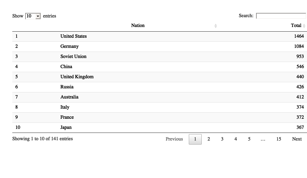
We now plot of the total number of medals awarded for each summer games in the period of 1960-2016.
nTotal <- medals_gm %>%
  group_by(Year) %>%
  summarise(TotalOfGames = sum(Total))
ggplot(nTotal, aes(x = Year, y = TotalOfGames)) + geom_line() + ylab("Total number of medals per Summer Games")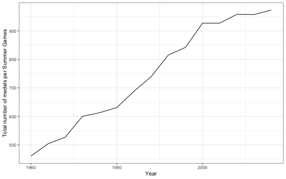
A distinct increasing trend is observed in the above figure. Hence,
in order to make between-country comparisons over time based on the
number of medals won, we normalize the medals by the total number of
medals awarded during the corresponding games. The result is stored in
the column Frac.
medals_gm <- medals_gm %>%
  left_join(nTotal, by = "Year") %>%
  mutate(Frac = Total / TotalOfGames)
After all these pre-processing steps, we can now compare country results for all summer games in the period 2000-2016.
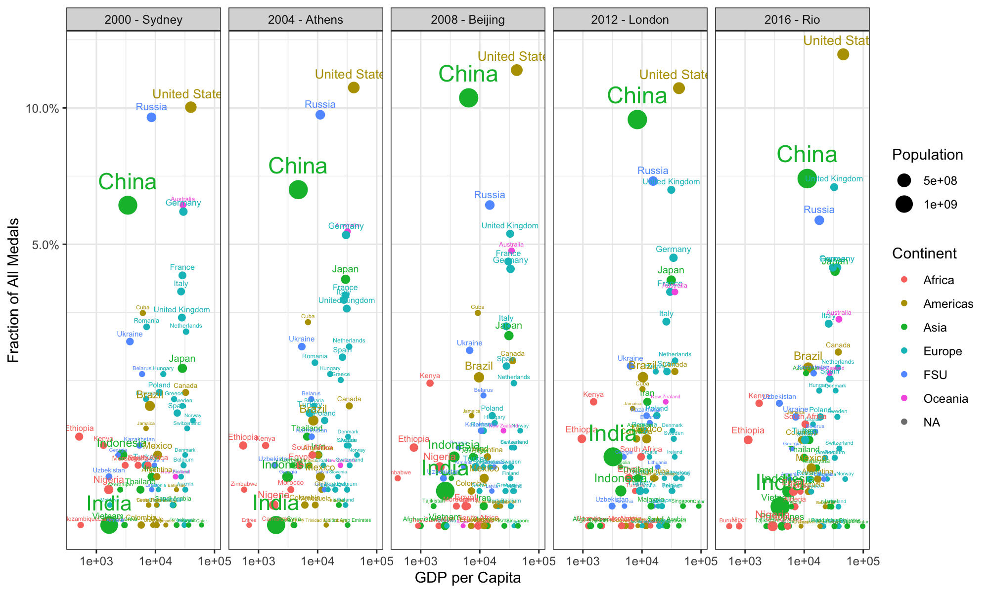
Note that for better visualization of the many countries with a small number of medals, an \(\sqrt{}\)-transform of the y-axis is used.
Finally, we can use the gganimate package to visualize
the dependence of the total number of medals won in the summer games
1960-2016 as a function of GDP per capita.
As before a \(\sqrt{}\)-transform of the y-axis is used for better visualization. One interesting observation we see from the animation is that the home-country of the Olympics always appears to do well in the following Olympics. Also note that the 1980 and 1984 were special due to boycotts. With respect to the top-5 nations it is also worth noticing that China, due to protests against the participation of Taiwan, did not participate in the Olympics 1956-1980. Furthermore, up to 1988 the team denoted “Germany” in the animation consists of the combined number of medals of “East Germany” and “West Germany”.
Fun with Flags
Update: After being made aware of the concurrent blog
entry by Philippe
Massicotte on how to visualize the Rio medal table using the
ggflags package, the above gapminder visualization can
easily be extended to use flags instead of nation names. As the
ggflags package only contains the flags of currently
existing countries we start the visualization in 1990. For better
visability we also add the trajectory of each nation.
Number of Medals per Population
To see the medal tables in a different light, we instead visualize a quantity relative to the number of medals per population. To enable cross-year comparisons we therefore compute the following index for each country and olympic summer games: \[ \frac{\text{Fraction of All Medals the Country got in that Year}}{\text{Population in the Country that Year}} \times 10^6. \] We shall call this index a country’s fraction of all medals per million population. A similar animation as above, now with logarithmic y-axis, illustrates the dynamics. To provide evidence supported neighbour mocking, we highlight the position of the three Nordic countries (Denmark, Sweden and Norway).
Jamaica, Bahamas and Grenada appear to do reasonably well lately compared to their population size. However, more more important - did you noticed the position of Denmark at the 2016 games in Rio?