Amazon's Hanging Cable Problem (Golden Gate Edition)
Abstract:
In this post we use R’s capabilities to solve nonlinear equation systems in order to answer an extension of the hanging cable problem to suspension bridges. We then use R and ggplot to overlay the solution to an image of the Golden Gate Bridge in order to bring together theory and practice.
 This work is licensed under a Creative Commons
Attribution-ShareAlike 4.0 International License. The
markdown+Rknitr source code of this blog is available under a GNU General Public
License (GPL v3) license from github.
This work is licensed under a Creative Commons
Attribution-ShareAlike 4.0 International License. The
markdown+Rknitr source code of this blog is available under a GNU General Public
License (GPL v3) license from github.
Introduction
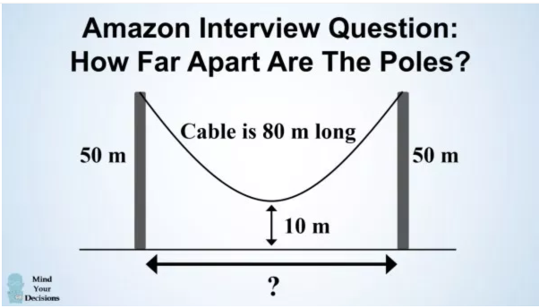
The so called Amazon’s hanging cable problem explained in this youtube video (watched 2.4 mio times!1) goes as follows:
A cable of 80 meters (m) is hanging from the top of two poles that are both 50 m from the ground. What is the distance between the two poles, to one decimal place, if the center of the cable is:
- 20 m above the ground?
- 10 m above the ground?
Hint: The solution to (a) is concisely described in Chatterjee and Nita (2010) and for (b) you need to do little more than just think. So instead of applying at Amazon, let’s take the question to the next level: Apply for the orange belt in R: How you wouldn’t solve the hanging cable problem by instead solving the hanging cable problem suspension bridge style!
As explained in the video the catenary curve is the geometric shape, a cable assumes under its own weight when supported only at its ends. If instead the cable supports a uniformly distributed vertical load, the cable has the shape of a parabolic curve. This would for example be the case for a suspension bridge with a horizontal suspended deck, if the cable itself is not too heavy compared to the road sections. A prominent example of a suspension bridges is the Golden Gate Bridge, which we will use as motivating example for this post.
Solving the Cable Problem
Parabola Shape
Rephrasing the cable problem as the ‘suspension bridge problem’ we need to solve a two-component non-linear equation system:
the first component ensures that the parabolic curve with vertex at \((0,0)\) goes through the poles at the x-values \(-x\) and \(x\). In other words: the distance between the two poles is \(2x\). Note that the coordinate system is aligned such that the lowest point of the cable is at the origo.
the second component ensures that the arc-length of the parabola is as given by the problem. Since the parabola is symmetric it is sufficient to study the positive x-axis
The two criteria are converted into an equation system as follows: \[ \begin{align*} a x^2 &= 50 - \text{height above ground} \\ \int_0^x \sqrt{1 + \left(\frac{d}{du} a u^2\right)^2} du &= 40. \end{align*} \]
Here, the general equation for arc-length of a function \(y=f(u)\) has been used. Solving the arc-length integral for a parabola can either be done by numerical integration or by solving the integral analytically or just look up the resulting analytic expression as eqn 4.25 in Spiegel (1968). Subtracting the RHS from each LHS gives us a non-linear equation system with unknowns \(a\) and \(x\) of the form
\[ \left[ \begin{array}{c} y_1(a,x) \\ y_2(a,x) \end{array} \right] = \left[ \begin{array}{c} 0 \\ 0 \end{array} \right]. \]
Writing this in R code:
## Height of function at the location x from center is (pole_height - height_above_ground)
y1_parabola <- function(a, x, pole_height=50, above_ground=20) {
  a*x^2 - (pole_height - above_ground)
}

## Arc-length of the parabola between [-x,x] is given as cable_length
y2_parabola <- function(a,x, cable_length=80, arc_method=c("analytic","numeric")) {

  ##Arc-length of a parabola a*u^2 within interval [0,x]
  if(arc_method == "numeric") {
    f <- function(u) return( sqrt(1 + (2*a*u)^2))
    half_arclength <- integrate(f, lower=0, upper=x)$value
  } else if (arc_method=="analytic") {
    half_arclength <-  1/(4*a)*(2*a*x*sqrt(4*a^2*x^2+1) + asinh(2*a*x))
  }

  ##The equation: s = cable_length/2
  half_arclength - cable_length/2
}

## The non-linear equation system \bm{y}(\theta) = \bm{0}, where the LHS
## is given by a list with two components containing y_1(\theta) and y_2(\theta)
f_sys <- function(theta, y, pole_height=50, above_ground=20, cable_length=80, ...) {
  ##Parameters
  a <- theta[1]
  x <- exp(theta[2]) ##ensure x is positive

  c(y[[1]](a,x, pole_height=pole_height, above_ground=above_ground),
    y[[2]](a,x, cable_length=cable_length, ...))
}

##Helper function to transform theta parameter vector to (a,x)'
theta2ax <- function(theta) {
  c(a=theta[1], x=exp(theta[2]))
}
To ensure \(x>0\) we
re-parametrized the equations with \(\theta_2
= \log(x)\) and provide the function theta2ax to
backtransform the result. We can now use the nleqslv
package to solve the non-linear equation system using a one-liner:
y_parabola <- list(y1_parabola, y2_parabola)
sol_parabola <- nleqslv(x=c(0.1,0.1),f_sys, y=y_parabola,  arc_method="analytic")
theta2ax(sol_parabola$x)
## a x
## 0.05355207 23.66859605In other words, for a cable of length 80m the pole of a suspension bridge will be located 23.7m from the origo, which means the two poles of the bridge will be 47.3m apart, which is also the span of the bridge.
Using arc_method="numeric" instead of the analytic
solution gives
##           a           x
## 0.05355207 23.66859605It is re-assuring to see that the numerical integration method yields the same result as the analytic method. The analytic method has mathematical beauty, the numerical method allows the data scientist to solve the problem without diving into formula compendiums or geometry.
Catenary Shape
Using the same code, but with the y-functions formulated for the catenary case we obtain
## Value of y=f(u) evaluated at u=x
y1_catenary <- function(a,x, pole_height=50, above_ground=20) {
  a * cosh(x/a) - a - (pole_height- above_ground)
}
## Arc-length condition
y2_catenary <- function(a,x, cable_length=80) {
  a * sinh(x/a) - cable_length/2
}

## Solve equation system
y_catenary <- list(y1_catenary, y2_catenary)
sol_catenary <- nleqslv(x=c(0.1,0.1),f_sys, y=y_catenary, method="Newton")
theta2ax(sol_catenary$x)
## a x
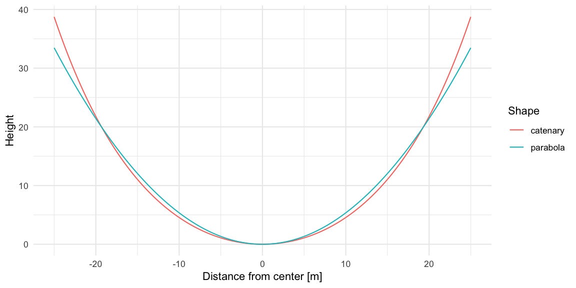
## 11.66667 22.70229In other words the solution to the original cable problem is \(x=22.7 m\) whereas the answer to the suspension bridge version is \(x=23.7m\). The difference to the parabolic form can be seen from the following graph:
Testing the theory
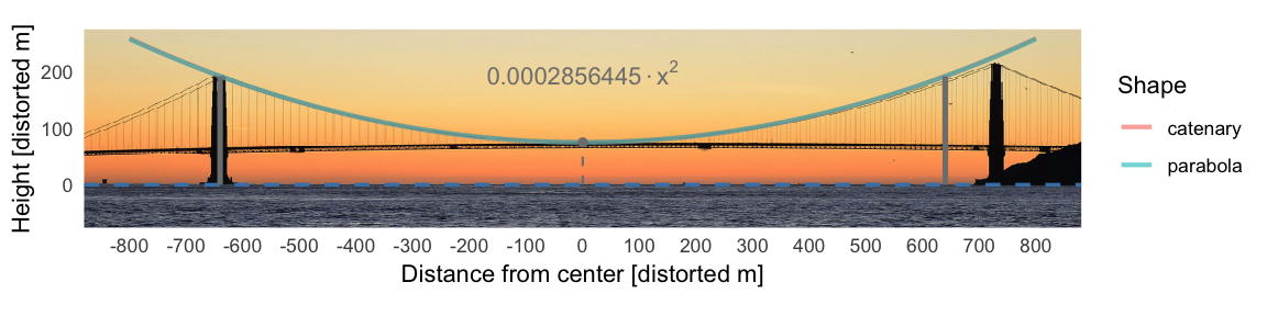
We test our theory by studying the cable of the Golden Gate
suspension bridge. Shown below is a photograph by D
Ramey Logan available under a CC BY 4.0
license. For presentation in this post the image was tilted by -0.75
degrees (around the camera’s view axis) with the imager
package to make the sea level approximately horizontal. Parabolic and
catenary overlays (no real difference between the two) were done using
the theory described above.
##Preprocess image
img <- imager::load.image(file.path(fullFigPath, "Golden_Gate_Bridge.png"))
img <- imager::imrotate(img, angle=-0.75, interpolation=1)
img <- imager::resize(img,-50,-50, interpolation_type=5)
We manually identify center, sea level and poles from the image and
use annotation_raster
to overlay the image on the ggplot of the corresponding
parabola and catenary. See the code
on github for details.
The fit is not perfect, which is due to the camera’s direction not being orthogonal to the plane spanned by the bridge - for example the right pole appears to be closer to the camera than the left pole2. We scaled and ‘offsetted’ the image so the left pole is at distance 640m from origo, but did not correct for the tilting around the \(y\)-axis. Furthermore, distances are being distorted by the lens, which might explain the poles being too small. Rectification and perspective control of such images is a photogrammetric method beyond the scope of this post!
Discussion
This post may not to impress a Matlab coding engineer, but it shows how R has developed into a versatile tool going way beyond statistics: We used its optimization and image analysis capabilities. Furthermore, given an analytic form of \(y(\theta)\), R can symbolically determine the Jacobian and, hence, implement the required Newton-Raphson solving of the non-linear equation system directly - see the Appendix. In other words: R is also a full stack mathematical problem solving tool!
As a challenge to the interested reader: Can you
write R code, for example using imager, which automatically
identifies poles and cable in the image and based on the known
specification of these parameters of the Golden Gate Bridge (pole
height: 230m, span 1280m, clearance above sea level: 67.1m), and perform
a rectification of the image? If yes, Stockholm University’s Math
Department hires
for Ph.D. positions every April! The challenge could work well as
pre-interview project. 😉
Appendix - Newton-Raphson Algorithm
Because the y_1(a,x) and y_2(a,x) are both
available in closed analytic form, one can form the Jacobian of
non-linear equations system by combining the two gradients. This can be
achieved symbolically using the deriv or Deriv::Deriv
functions in R.
Given starting value \(\theta\) the iterative procedure to find the root of the non-linear equation system \(y(\theta) = 0\) is given by (Nocedal and Wright 2006, Sect. 11.1)
\[ \theta^{(k+1)} = \theta^k - J(\theta^k)^{-1} y(\theta), \]
where \(J\) is the Jacobian of the system, which in this case is a 2x2 matrix.
gradient_y1 <- Deriv::Deriv(y1_parabola, x=c("a","x"))
y2_parabola_analytic <- function(a,x, cable_length=80) {
1/(4*a)*(2*a*x*sqrt(4*a^2*x^2+1) + asinh(2*a*x)) - cable_length/2
}
gradient_y2 <- Deriv::Deriv(y2_parabola_analytic, x=c("a","x"))
##Jacobian
J <- function(theta, pole_height=50, above_ground=20, cable_length=80, ...) {
a <- theta[1]
x <- exp(theta[2]) # x <- exp(theta[2])
##Since we use x = exp(theta[2])=g(theta[2]) we need the chain rule to find the gradient in theta
##this is g'(theta[2]) = exp(theta[2]) = x
rbind(gradient_y1(a,x, pole_height=pole_height, above_ground=above_ground)* c(1, x),
gradient_y2(a,x, cable_length=cable_length) * c(1, x))
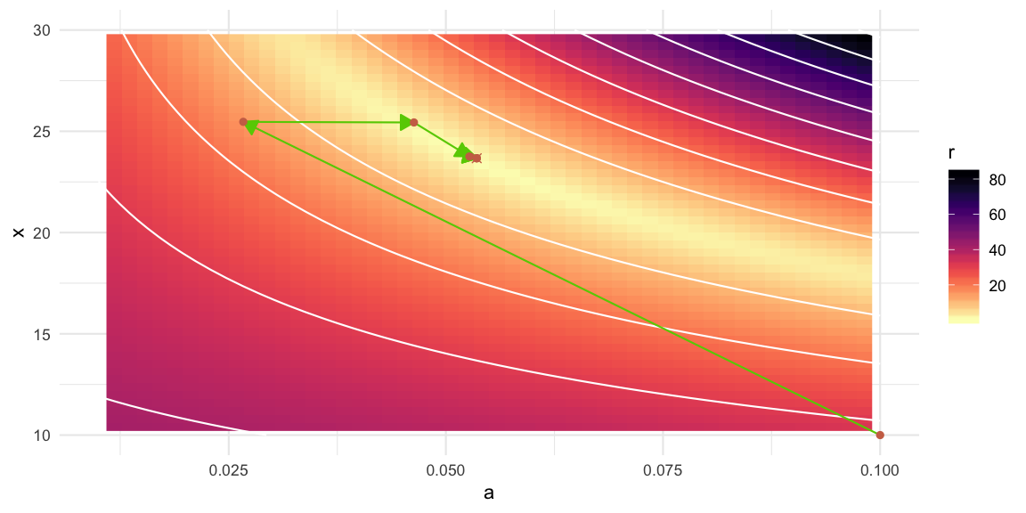
}By iterating Newton-Raphson steps we can find the solution of the equation system manually:
##Start values
theta <- c(0.1,log(10))
thetanew <- c(0.1,log(20))
##Log with the values
log <- t(theta2ax(theta))

##Iterate Newton-Raphson steps until convergence
while ( (sum(thetanew - theta)^2 / sum(theta^2)) > 1e-15) {
  theta <- thetanew
  ##Update step
  thetanew <- theta - solve(J(theta=theta)) %*% f_sys(theta, y=y_parabola, arc_method="analytic")
  ##Add to log
  log <- rbind(log, theta2ax(thetanew))
}

##Look at the steps taken
log
## a x
## [1,] 0.10000000 10.00000
## [2,] 0.02667392 25.46647
## [3,] 0.04632177 25.43589
## [4,] 0.05270610 23.75416
## [5,] 0.05354318 23.66953
## [6,] 0.05355207 23.66860
## [7,] 0.05355207 23.66860We show the moves of the algorithm in a 2D contour plot for \(r(a,x) = \sqrt{y_1(a,x)^2 + y_2(a,x)^2}\). The solution to the system has \(r(a,x)=0\). See the code on github for details.