Safe Disposal of Unexploded WWII Bombs
Abstract
Unexploded WWII bombs are ticking threats despite being dropped more
than 70 years ago. In this post we explain how statistical methods are
used to plan the search and disposal of unexploded WWII bombs. In
particular we consider and exemplify the non-parametric nearest
neighbour distance (NND) method implemented in the R package
highriskzone. The method analyses the spatial pattern of
exploded bombs to determine so called risk-zones, that is regions with a
high likelihood of containing unexploded bombs. The coverage of such
risk-zones is investigated through both non-parametric and parametric
point process simulation.

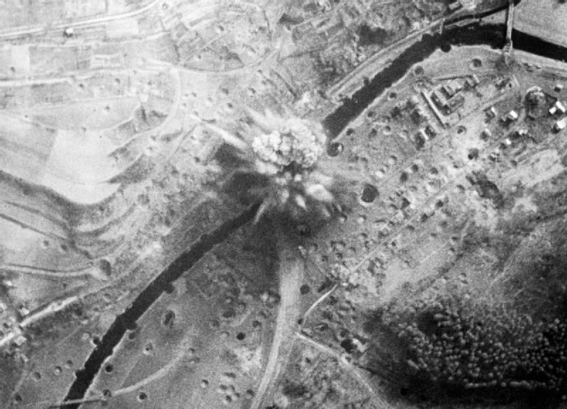
NCAP aerial photo from 1944 showing the bombing of the V2 rocket facility at Peenemünde, Germany. Image is available under a custom NCAP license - higher resolution images are available from NCAP.
 This work is licensed under a Creative Commons
Attribution-ShareAlike 4.0 International License. The
markdown+Rknitr source code of this blog is available under a GNU General Public
License (GPL v3) license from github.
\[ \newcommand{\bm}[1]{\boldsymbol{\mathbf{#1}}} \]
Introduction
During WWII Germany was pounded with about 1.5 mio tons of bombs of which about 10-15% did not explode. More than 70 years after the end of WWII these unexploded bombs (UXBs) still pose a threat and are the frequent cause of large scale evacuations to secure their safe disposal when found. Luckily, lethal incidents are rare thanks to a huge effort to localise and safely dismantle UXBs. As part of this effort, aerial photos taken by the allies after the attacks provide valuable information about the possible locations of UXBs. Some UXBs are directly visible in the photos - see for example the green circles in this NCAP image or p. 6 in the following information flyer by one of the companies offering such aerial identification services (featured in this news article). In other cases the photos only provide information about the location of the exploded bombs. This information can be used to identify areas where there is a high likelihood of UXBs. Such areas would then be carefully scrutinized using on-the-ground search methods, for example, electromagnetic and magnetic detectors.
The aim of Mahling, Höhle, and Küchenhoff
(2013) was to develop statistical methods for the identification
of such risk-zones in co-operation with Oberfinanzdirektion
Niedersachsen, which supports the removal of unexploded ordnance in
federal properties in Germany. In what follows we will discuss
one of the methods used in the paper, the so called
nearest neighbourhood distance method and illustrate
its implementation in the R package highriskzone originally
created by Heidi Seibold and
now maintained by Felix
Günther.
Mathematical Setup
Casting matters into mathematical notation: Let \(X\) be a point process denoting the spatial locations of all bombs dropped in the particular window of interest \(W \subseteq \mathbb{R}^2\). Furthermore, let \(Y\) denote the observed point process of exploded bomb and \(Z=X\backslash Y\) the point process of unexploded bombs. Note that only the process \(Y\) is observed; \(Z\) is not observed and the target of our inference. We assume that the probability \(q\) of a dropped bomb not exploding is homogeneous in \(W\). Thus if \(X\) is a inhomogeneous Poisson point process with intensity function \(\lambda_X(\bm{s})\), \(\bm{s}\in W\), then
\[ \lambda_Y(\bm{s}) = (1-q) \lambda_X(\bm{s}) \quad \text{and}\quad \lambda_Z(\bm{s}) = q \lambda_X(\bm{s}) \]
are the intensity functions of \(Y\) and \(Z\), respectively.
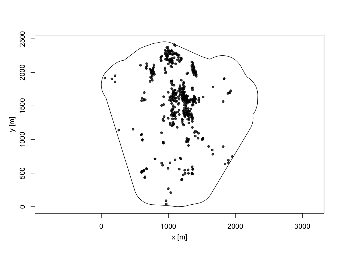
The figure below shows \(Y\) for an
actual observed WWII bomb point consisting of n=443 bombs available from
the R package highriskzone (Seibold et al. 2017). The observation
window contains a particular area of interest for which a risk
assessment needs to be done - often these contain a known WWII military
target, e.g., an airport, an arms factory or a military casern. In order
to not disclose the exact location of the considered area, coordinates
are given relative to an arbitrary origo. In reality one would closely
link such digitized aerial images to other terrain features using a GIS
system.
library(highriskzone)
library(spatstat)
data(craterA)
summary(craterA)
## Planar point pattern: 443 points
## Average intensity 0.0001082477 points per square unit
##
## Coordinates are given to 4 decimal places
##
## Window: polygonal boundary
## single connected closed polygon with 208 vertices
## enclosing rectangle: [0, 2334.3758] x [0, 2456.4061] units
## Window area = 4092470 square units
## Fraction of frame area: 0.714 The point pattern
 craterA corresponding to an instance of
the process \(Y\) is provided in R as
an object of class ppp from the R package spatstat (Baddeley, Rubak, and
Turner 2015). Instead of inferring the locations in \(Z\) directly, we shall be interested in
determining a region within \(W\), a so
called high risk zone, which with a high likelihood
contains the points of \(Z\). We shall
consider two methods for this job: a non-parametric method based on
nearest neighbour distances in \(Y\)
and an intensity function based inhomogeneous Poisson process approach
incorporating \(q\).
High Risk Zones
A heuristic way to determine a high-risk zone is the following: Determine the distribution function \(D\) of the nearest neighbour distance (NND) distribution based on the 443 points in the point pattern. Use the distribution to determine a desired quantile, say \(0 \leq p \leq 1\) of the NND distribution. Denoting the \(p\) sample quantile of the NND distribution by \(Q(p)\), a \(p\)-quantile NND based high-risk zone is then obtained as the union of putting a disc of radius \(x_q\) around each observed exploded bomb in \(Y\) - in mathematical terms:
\[ R_p = \left(\bigcup_{\bm{y} \in Y} B(\bm{y}, Q(p))\right) \bigcap W = \left\{\bm{s} \in W : \min_{\bm{y}\in Y} || \bm{s} − \bm{y} || \leq Q_Y(p) \right\}, \]
where \(B(\bm{s}, r)\) denotes a
disc of radius \(r\) around the point
\(\bm{s}\) and \(||\bm{s} - \bm{y}||\) is the distance
between the two points \(\bm{s}\) and
\(\bm{y}\). The intersection with \(W\) is done in order to guarantee that the
risk zone lies entirely within \(W\).
As an example, we would determine the 99%-quantile NND zone for
craterA using spatstat functionality as
follows:
(Qp <- quantile(nndist(craterA), p = 0.99, type = 8))## 99%
## 142.1391dmap <- distmap(craterA)
zone_dist <- eval.im( dmap < Qp )The above can also be done directly using
highriskzone::det_hrz function:
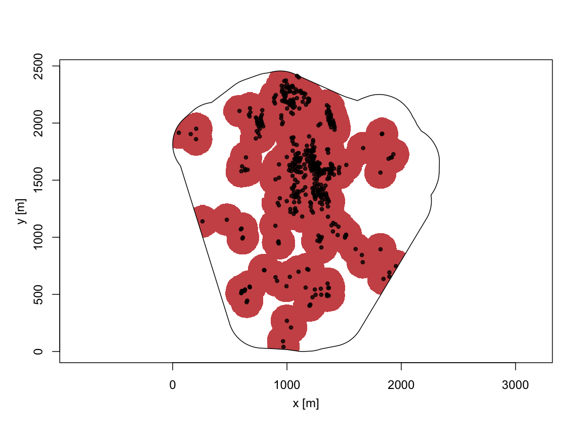
zone_dist <- det_hrz(craterA, type="dist", criterion = "indirect", cutoff=0.99)Either way, the resulting risk-zone is as follows:
summary(zone_dist)## high-risk zone of type dist
## criterion: indirect
## cutoff: 0.99
##
## threshold: 142.1391
## area of the high-risk zone: 2580654 Mahling, Höhle, and
Küchenhoff (2013) show that risk zones constructed by the NND
method work surprisingly well despite lacking a clear theoretical
justification. One theoretical issue is, for example, that the NND
distribution function determined by the above method is for the \((1-q)\) thinned process \(Y\), even though the actual interest is in
the process \(X=Y\cup Z\). Because of
the thinning one would typically have that \(D_Y(r) \leq D_X(r)\) and thus \(Q_Y(p) > Q_X(p)\). Using \(Q_Y(p)\) to make statements about \(X\) (and thus \(Z\)) is therefore slightly wrong. However,
this error cancels, because we then use the points in \(Y\) to add a buffer of radius \(Q_Y(p)\). Had we instead used the smaller,
but true, \(Q_X(p)\) the risk zone
would have gotten a too small, because \(X\) would also have contained more points
to form discs around than \(Y\). The
method thus implicitly takes \(q\)
non-parametrically into account, because its NND is determined based on
\(Y\) and subsequently discs of radius
\(Q_Y(p)\) are formed around the points
of \(Y\).
Technical details you might want to skip: The above feature is most easily illustrated if \(X\) is a homogeneous Poisson process with intensity \(\lambda_X\). In this case we have that the NND distribution function is (p.68, Illian et al. 2008)
\[ D_X(r) = 1 - \exp(-\lambda_X \pi r^2), \quad r>0. \]
Also note that \(D_Y(r) = 1 - \exp(-(1-q)\lambda_X \pi r^2)\) and therefore \(D_Y(r) > D_X(r)\). Now solving for the \(p\)-quantile of the NND in this homogeneous Poisson case means solving
\[ Q_Y(p) = \min_{r\geq 0} \{ D_Y(r) \geq p \} \Leftrightarrow Q_Y(p) = \sqrt{ \frac{\log(1-p)}{\lambda_Y \pi}}. \]
From this it becomes clear than in the homogeneous Poisson case \(Q_ Y(p)\) is a factor \(\sqrt{1/(1-q)}\) larger than \(Q_X(p)\), which is the actual target of interest.
Assessing the coverage of a risk-zone
Two criterion appear immediate in order to assess the coverage of a risk-zone \(R\):
The probability \(p_{\text{out}}\) that there will be at least one bomb outside the risk zone, i.e. \(P( N( Z \backslash R) > 0)\), where \(N(A)\) denotes the number of events in the set \(A \subseteq W\). Note: this probability is depending heavily on the amount of points in \(Z\), the more points there are, the higher is \(p_{\text{out}}\). However, it reflects the idea “one miss is all it takes to get in trouble”.
The proportion of events in \(Z\) not located in \(R\), i.e. \(N( Z \backslash R) / N(Z)\), we shall denote this criterion by \(p_{\text{miss}}\). Note: This probability is taking possible different sizes of \(Z\) into account, but also takes a more relative approach towards how many bombs are not covered by the zone.
Under the assumption of independence between whether \(Z\)-events are within or outside the risk-zone one can convert back and forth between \(p_{\text{miss}}\) and \(p_{\text{out}}\) by
\[ p_{\text{out}} = P( N( Z \backslash R) > 0) = 1- P(N(Z \backslash R) = 0) \approx 1 - (1-p_{\text{miss}})^{N(Z)}, \]
where one in a simulation setup would know \(Z\) and thus also \(N(Z)\). Note that for a \(p\)-quantile NND risk-zone we expect \(1-p_{\text{miss}}\) to be approximately equal to \(p\). We can investigate the behaviour of risk-zones according to the two above criterion through the use of simulation. Either by simply \(q\)-thinning of the existing point pattern \(Y\) and then use this thinned pattern to determine a risk-zone, which is then evaluated. An alternative approach is to estimate the intensity surface from \(Y\), upscale it to get the intensity of \(X\), simulate \(X\) as an inhomogeneous Poisson point process with this intensity surface, thin this pattern to get a simulated instance of \(Y\), construct the risk-zone based on this pattern and then evaluate the coverage of the zone (Mahling, Höhle, and Küchenhoff 2013). Note that this type of simulation is based on more assumptions compared to the non-parametric thinning simulation approach.
We generate 1,000 realizations of \(Y\) and \(Z\) through \(q\)-thinning of the original
craterA pattern while computing the coverage measures for
the NND method as follows:
suppressPackageStartupMessages(library(doParallel))
registerDoParallel(cores=4)

simulate_method <- "thinning" #"intensity" # "cond_intensity"
sim <- foreach(i=seq_len(getDoParWorkers()), .combine=rbind) %dopar% {
  tryCatch(
    eval_method(craterA, type=c("dist"), criterion=c("indirect"),
                cutoff=0.99, numit = 250, simulate=simulate_method,
                pbar=FALSE),
    error= function(e) return(NULL))
}
## # A tibble: 1 x 5
## p_out p_miss `1-p_miss` p_out_derived nZ
## <dbl> <dbl> <dbl> <dbl> <dbl>
## 1 0.097 0.00236 0.998 0.0996 44.4The numbers state the average p_out and
p_missin the 1000 simulations. Furthermore, nZ
denotes the average number of events in \(Z\). We see that the NND method performs
even a little better than intended, because \(1-p_{\text{miss}}\) is even higher than the
intended \(p\)=99%. The probability
that the risk-zone misses at least one bomb lies as low as 0.097. This
is quite close to the above described approximate conversion from \(p_{\text{miss}}\) (0.100 vs. 0.097).
Changing the simulation method for \(X\) to that of an inhomogeneous Poisson
process with intensity \(1/(1-q) \cdot
\hat{\lambda}_Y(\bm{s})\) yields similar results:
## # A tibble: 1 x 5
##   p_out  p_miss `1-p_miss` p_out_derived    nZ
##   <dbl>   <dbl>      <dbl>         <dbl> <dbl>
## 1 0.352 0.00897      0.991         0.361  49.6
We note that the probability of missing at least one bomb is much higher under this parametric simulation method. Only a small fraction of this is explained by \(Z\) now consisting of more points. A likely explanation is that the parametric model is only semi-adequate to describe how the point patterns form. Therefore, the new \(X\) might have a somewhat different neighbourhood distribution than anticipated.
To compare more specifically with the intensity function based risk-zone method of Mahling, Höhle, and Küchenhoff (2013) we use a specification, where the risk-zone derived by the NND method or the intensity method have the same area (250 hectare).
sim_area <- foreach(i=seq_len(getDoParWorkers()), .combine=rbind) %dopar% {
  tryCatch(
    eval_method(craterA, type=c("dist","intens"), criterion=rep("area",2),
                cutoff=rep(2500000,2), numit = 100,
                simulate=simulate_method, pbar=FALSE),
    error= function(e) return(NULL))
}
## # A tibble: 2 x 6
## Type p_out p_miss `1-p_miss` p_out_derived area_zone
## <fct> <dbl> <dbl> <dbl> <dbl> <dbl>
## 1 dist 0.123 0.00278 0.997 0.117 2500009.
## 2 intens 0.55 0.0172 0.983 0.539 2499994.For the particular example we see an advantage of using the NND
method, because both p_out p_miss are much
lower for the intensity based method. Again, this might be due to the
intensity method being based on assumptions, which for the particular
example do not appear to be so adequate. Results in Mahling (2013) were,
however, much better for this example (c.f. Tab 2), which could be an
indication that there is a problem in the highriskzone
package implementation of this method?
Discussion
Being a statistician is fascinating, because the job is the entry ticket to so many diverse research fields. The proposed methods and evaluations helped the Oberfinanzdirektion obtain a quantitative framework to decide which methods to use in their routine risk-assessment. Further details on the above application can be found in Mahling, Höhle, and Küchenhoff (2013) as well as in Monia’s Ph.D. dissertation (Mahling 2013). Note also that the techniques are not limited to UXB detection: Infer-unknown-points-from-a-thinned-process problems occur both in 1D and 2D point processes in a range of other fields, e.g., under-reporting of infectious disease locations or in the calculation of animal abundance in ecology.
As a personal anecdote: When finishing the work on Mahling, Höhle, and Küchenhoff (2013) I was in transition from university to working at a public health institute. The deal was to finish the UXB work partly in spare-time and partly in the new work time. To honour this I added my new work place as second affiliation before submitting, but as part of the institution’s internal clearing procedure of the publication, I was asked to remove this affiliation again by the higher management, because the work ‘had nothing to do with public health’. While its questionable whether exploding bombs really do not have a public health impact, a few months later, I ended up using very similar statistical techniques to model occurred-but-not-yet-reported cases during a critical infectious disease outbreak (Höhle and an der Heiden 2014).
