Right or Wrong? - Validate Numbers Like a Boss
Abstract
How does a statistician ensure that an analysis that comprises of outputting \(N\) results is correct? Can this be done without manually checking each of the results? Some statistical approaches for this task of proof-calculation are described - e.g. capture-recapture estimation and sequential decision making.
 This work is licensed under a Creative Commons
Attribution-ShareAlike 4.0 International License. The
markdown+Rknitr source code of this blog is available under a GNU General Public
License (GPL v3) license from github.
This work is licensed under a Creative Commons
Attribution-ShareAlike 4.0 International License. The
markdown+Rknitr source code of this blog is available under a GNU General Public
License (GPL v3) license from github.
Introduction
One activity the public associates with statistics is the generation of large tables containing a multitude of numbers on a phenomena of interest. Below an example containing the summary of UK labour market statistics for the 3 months to February 2016 from the Office for National Statistics:

Another example is The German Federal Government’s 4th Report on Poverty and Wealth. The report consists of a total of 549 pages with the pure table appendix fun starting on p. 518 including, e.g., age-adjusted ORs obtained from logistic regression modelling (p.523).
Even though dynamic & web-based reporting coupled with graphical & interactive visualizations have developed to a point making such tables obsolete, this does not change the fact that the results still need to be correct. As a consequence, the results need to be validated to ensure their correctness, occasionally even beyond any doubt! In what follow we will use the term result to describe an output element of the statistical analysis. In most cases results are numbers, but we shall use the term number and result interchangeably. However, results could also denote higher level output elements, e.g., complete tables, a specific line in a graph or the complete output of a particular query.
Surprisingly, statistics students are taught very little about
addressing such a task using what we do best: statistics. We teach about
the median, censoring & truncation, complex modelling and computer
intensive inference methods. Maybe we even tell them about
knitr as way to get the same results twice (a minimum
requirement to ensure correctness). However, spraying out numbers (even
from the most beautiful model) is not cool if the
initial data-munging went wrong or if your quotient is obtained by
dividing with the wrong denominator.
The on-going discussion of reproducible research aims at the core of this problem: How to ensure that your analysis re-producible and correct? As modern statistics becomes more and more programming oriented it appears natural to seek inspiration from the discipline of software testing. Another entertaining source of inspiration is the concept of optimal proofreading. This dates back to the 1970-1980s, where the problem is formulated as the search for an optimal stopping rules for the process of checking a text consisting of \(M\) words - see for example Yang et al. (1982). Periodically, the software development community re-visits these works - see for example Hayes (2010). Singpurwalla and Wilson (1999) give a thorough exposition of treating uncertainty in the context of software engineering by interfacing between statistics and software engineering.
Proofcalculation
The scientific method of choice to address validity is peer review. This can go as far as having the reviewer implement the analysis as a completely separate and independent process in order to check that results agree. Reporting the results of clinical trials have such independent implementations as part of the protocol. Such a co-pilot approach fits nicely to the fact that real-life statistical analysis rarely is a one-person activity anymore. In practice, there might neither be a need nor the resources to rebuild entire analyses, but critical parts need to be double-checked. Pair programming is one technique from the agile programming world to accomodate this. However, single programmers coding independently and then compare results appears a better way to quality-control critical code & analysis segments.
Formalizing the validation task into mathematical notation, let’s assume the report of interest consists of a total of \(N\) numbers. These numbers have a hierarchical structure, e.g., they relate to various parts of the analysis or are part of individual tables. Error search is performed along this hierarchical structure. Good proofcalculation strategies follow the principles of software testing - for example it may be worthwhile to remember Pareto’s law: 80 percent of the error are found in 20 percent of the modules to test. In other words: keep looking for errors at places where you already found some. Further hints on a well structured debugging process can be found in Zeller (2009) where the quote on Pareto’s law is also from.
One crucial question is what exactly we mean by an error? A result can be wrong, because of a bug in the code line computing it. Strictly speaking wrong is just the (mathematical) black-and-white version of the complex phenomena describing a misalignment between what is perceived and what is desired by somebody. A more in-depth debate of what’s wrong is beyond the scope of this note, but certainly there are situations when a result is agreeably wrong, e.g., due to erroneous counting of the number of distinct elements in the denominator set. More complicated cases could be the use of a wrong regression model compared to what was described in the methodology section, e.g., use of an extra unintended covariate. Even worse are problems in the data-prepossessing step resulting in a wrong data foundation and, hence, invalidating a large part of the results. Altogether, a result be wrong in more than one way and one error can invalidate several results: the \(M\) results are just the final output - what matters is what happens along your analysis pipeline. Detecting a wrong result is thus merely a symptom of a flawed pipeline. This also means that fixing the bug causing a number to be wrong does not necessarily ensure that the number is correct afterwards.
We summarise the above discussion by making the following simplifying abstractions:
The number of results which is wrong is a function of the number of errors \(M\). One error invalidates at least one result, but it can invalidate several jointly and errors can overlap thus invalidating the same number.
We deliberately keep the definition of an error vague, but mean a mechanism which causes a result to be wrong. The simplest form of a result is a number. The simplest error is a number which is wrong.
The hierarchical structure of the numbers and the intertwined code generating them is ignored. Instead, we simply assume there are \(M\) errors and assume that these errors are independent of each other.
We shall now describe an estimation approach a decision theoretic approach for the problem.
Team Based Validation
Consider the situation where a team of two statisticians together validate the same report. Say the team use a fixed amount of time (e.g. one day) trying to find as many errors in the numbers as possible. During the test period no errors are fixed - this happens only after the end of the period. Let’s assume that during the test period the two statistician found \(n_1\) and \(n_2\) wrong numbers, respectively. Let \(0 \leq n_{12} \leq \min(n_1,n_2)\) be the number of wrong numbers which were found by both statisticians.
The data in alternative representation: Denote by \(f_i, i=1,2\) the number of wrong numbers found by \(i\) of the testers, i.e.
\[ \begin{aligned} f_1 &=(n_1-n_{12})+(n_2-n_{12})\\ f_2 &= n_{12}. \end{aligned} \]
These are the wrong numbers found by only one of the testers and by both testers, respectively. Let \(S=f_1+f_2=n_1+n_2-n_{12}\) be the total number of erroneous numbers found in the test phase. Assuming that we in the subsequent debugging phase are able to remove all these \(S\) errors, we are interested in estimating the number of remaining errors, i.e. \(f_0\) or, alternatively, the total number of errors \(M=S+f_0\).
Assume that after the first day of proofcalculation the two statisticians obtain the following results:
testP <- data.frame(t(c(9,12,6)))
colnames(testP) <- c("01","10","11")
testP
## 01 10 11
## 1 9 12 6i.e. \(n_1=9\), \(n_2=12\) and \(n_{12}=6\). The total number of errors
found so far is \(S=27\). In the above
code we use index 01, 10 and 11
specifying the results in two binary variable bit-notation - this is
necessary for the CARE1 package used in the next
section.
Estimating the total number of wrong numbers
Estimating the total number of errors from the above data is a capture-recapture problem with two time points (=sampling occasions).
Lincoln-Petersen estimator
Under the simple assumption that the two statisticians are equally good at finding errors and that the possible errors have the same probability to be found (unrealistic?) a simple capture-recapture estimate for the total number of errors is the so called Lincoln-Petersen estimator):
\[ \hat{M} = \frac{n_1 \cdot n_2}{n_{12}}. \]
Note that this estimator puts no upper-bound on \(N\). The estimator can be computed using,
e.g., the CARE1
package:
(M.hat <- CARE1::estN.pair(testP))## Petersen Chapman se cil ciu
## 45.000000 42.428571 9.151781 32.259669 72.257758In other words, the estimated total number of errors is 45. A 95% confidence interval (CI) for \(M\) is 32-72 - see the package documentation for details on the method for computing the (CI). To verify the computations one could alternatively compute the Lincoln-Petersen estimator manually:
(Nhat <- (testP["01"]+testP["11"]) * (testP["10"]+testP["11"]) / testP["11"])## 01
## 1 45Finally, an estimate on the number of errors left to find is \(\hat{M}-S=18.0\).
Heterogeneous Sampling Probabilities
If one does not want to assume the equal catch-probabilities of the errors, a range of alternatives exists. One of them is the procedure by Chao (1984, 1987). Here, a non-parametric estimate of the total number of errors is given as:
\[ \hat{M} = S + \frac{f_1^2}{2 f_2}. \]
The above estimator is based on the assumption that the two
statisticians are equally good at spotting errors, but unlike for the
Petersen-Lincoln estimator, errors can have heterogeneous detection
probabilities. No specific parametric model for the detection is
although required. An R implementation of the estimator is readily
available as part of the SPECIES
package. For this, data first need to be stored as a
data.frame containing \(f_1,
f_2\):
testPaggr <- data.frame(j=1:2,f_j=as.numeric(c(sum(testP[1:2]),testP[3])))
testPaggr
## j f_j
## 1 1 21
## 2 2 6(M_est <- SPECIES::chao1984(testPaggr, conf=0.95))## $Nhat
## [1] 64
##
## $SE
## [1] 22.78363
##
## $CI
## lb ub
## [1,] 39 139In this case the estimator for the total number of errors is \(\hat{M}\)=64 (95% CI: 39-139). Again see the package documentation for methodological details.
Knowing when to Stop
Whereas the above estimates are nice to know, they give little guidance on how, after the first day of testing, to decide between the following two alternatives: continue validating numbers for another day or stop the testing process and ship the report. We address this sequential decision making problem by casting it into a decision theoretic framework. Following the work of Ferguson and Hardwick (1989): let’s assume that each futher round of proofcalculation costs an amount of \(C_p>0\) units and that each error undetected after additional \(n\) rounds of proofcalculation costs \(c_n>0\) units. Treating the total number of wrong results \(M\) as a random variable and letting \(X_1,\ldots,X_n\), be the number of wrong results found in each of the additional proofcalculation rounds \(1,\ldots,n\), we know that \(X_i\in \mathbb{N}_0\) and \(\sum_{j=1}^n X_j \leq N\). One then formulates the conditional expected loss after \(n, n=0, 1, 2, \ldots,\) additional rounds of proofcalculation:
\[ Y_n = n C_p + c_n E(M_n|X_1,\ldots,X_n), \]
where \(M_n = M -(\sum_{j=1}^n X_j)\). If we further assume that in the \((n+1)\)’th proofcalculation round errors are detected independently of each other with probability \(p_n, 0 \leq p_n \leq 1\) and \(p_n\) being a known number we obtain that
\[ X_{n+1} \>|\> M, X_1,\ldots,X_n \sim \text{Bin}(M_n, p_n), \quad n=0,1,2,\ldots. \]
Under the further assumption that \(M\sim \text{Po}(\lambda)\) with \(\lambda>0\) being known, one can show that the loss function is independent of the observations (Ferguson and Hardwick, 1989), i.e.
\[ Y_n = n C_p + c_n \lambda \prod_{j=0}^{n-1} (1-p_j), \quad n=0,1,2,\ldots. \]
The above Poisson assumption seems to be an acceptable approximation if the total number of results \(M\) is large and the probability of a result being wrong is low. In this case the optimal stopping rule is given by:
\[ n_{\text{stop}} = \min_{n\geq 0} Y_n. \]
One limitation of the above approach is that we have used a guesstimate on how the detection probability \(p_n\) evolves over time. An extension would be to sequentially estimate this parameter from the obtained results. This goes along the lines of Dalal and Mallows (1988) which discuss when to stop testing your software - see the following blog entry for a short statistical treatment of their approach.
Numerical example
We consider a setup where the costly errors have substantial ramifications and thus are easy to detect early on. As time passes on the errors become more difficult to detect. This is reflected by the subsequent choices of \(p_n\) and \(c_n\) - see below. Furthermore, the expected number of bugs is taken to be the non-homogeneous capture-recapture estimate of the remaining errors. This coupling of the two procedures is somewhat pragmatic: it does not include the first round of proofcalculation in the decision making as this is used to estimate \(\lambda\). Furthermore, no estimation uncertainty in \(\lambda\) from this stage is transferred to the subsequent stages.
#Cost of one round of proofcalculation (say in number of working days)
Cp <- 1
#Cost of finding errors after n round of proofcalculation
cn <- function(n) 10*0.9^(2*(n+1))
#Expected number of errors
(lambda <- M_est$Nhat - sum(testP))
## [1] 37#Probabilty of detecting an error in round j+1
pj <- function(j) {
0.8^(j+1)
}
#Expected conditional loss as defined above
Yn <- Vectorize(function(n) {
n*Cp + cn(n) * lambda * prod(1-pj(0:(n-1)))
})
#Make a data.frame with the results.
df <- data.frame(n=1:20) %>% mutate(Yn=Yn(n),cn=cn(n),pn=pj(n-1))The above choice of parameters leads to the following functional forms:
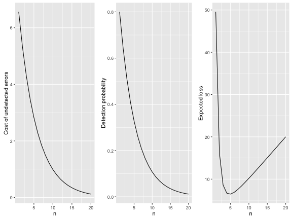
The optimal strategy is thus found as:
df %>% filter(rank(Yn) == 1) %>% select(n,Yn)## n Yn
## 1 5 6.457426In other words, one should test after \(n_{\text{stop}}=5\) additional rounds.
Discussion
Is any of the above useful? Well, I have not heard about such approaches being used seriously in software engineering. The presented methods narrow down a complex problem down using assumptions in order to make the problem mathematically tractable. You may not agree with the assumptions as, e.g., Bolton (2010) - yet, such assumptions are a good way to get started. The point is that statisticians appear to be very good at enlightening others about the virtues of statistics (repeat your measurements, have a sampling plan, pantomimic acts visualizing the horror of p-values). However, when it comes to our own analyses, we are surprisingly statistics-illiterate at times.

Literature
Bolton, M (2010). Another Silly Quantitative Model, Blog post, July 2010.
Cook, JD (2010). How many errors are left to find?, Blog post, July 2010.
Dalal, S. R. and C. L. Mallows. “When Should One Stop Testing Software?”. Journal of the American Statistical Association (1988), 83(403):872–879.
Ferguson, TS and Hardwick JP (1989). Stopping Rules For Proofreading, J. Appl. Prob. 26:304-313.
Hayes, B (2010). The thrill of the chase, Blog post, July 2010.
Singpurwalla ND, Wilson SP (1999). Statistical Methods in Software Engineering, Springer.
Yang MCK, Wackerly DD, Rosalsky A (1982). Optimal Stopping Rules in Proofreading, Journal of Applied Probability 19(3), pp. 723-729
Zeller, A (2009). Why programs fail, Elsevier, 2009, 423 pages.